Week 9 – Finalizing My Results: Confounding Variables, Multicollinearity, and Interactions
Welcome back to Week 9 of my senior project! This week, I’ve been finalizing my results, addressing multicollinearity, exploring potential lag effects over time, and running regression interactions to explain the seemingly contradictory results between my initial findings and my results after controlling for confounding variables.
Multicollinearity
Multicollinearity occurs when two or more independent variables in a regression model are highly correlated, making it difficult to determine their individual effects on the dependent variable. When this happens, our model might produce misleading conclusions.
How can we detect and solve for multicollinearity?
One of the most common ways to detect multicollinearity is by using the Variance Inflation Factor (VIF). VIF measures how much a variable’s variance is inflated due to collinearity with other predictors in the model. Because many of my variables are categorical and have more than 1 degree of freedom, I will be using Adjusted Generalized Variance Inflation Factor (GVIF^(1/(2*Df))
GVIF Interpretation:
- GVIF = 1 → No correlation (ideal)
- GVIF > 2 → Moderate to strong multicollinearity (should remove variable from model)
My GVIF Results:
| Variable | GVIF^(1/(2*Df) |
| Sex | 1.057 |
| Age | 1.471 |
| Education | 1.652 |
| Race/Ethnicity | 1.061 |
| Income | 1.543 |
| Years in the U.S. | 1.095 |
| Occupation Type | 2.512 |
| Industry | 1.089 |
| Region | 1.011 |
| Year | 1.001 |
In the table above, we can see that the adjusted GVIF for occupation type is very high (about 2.5). Intuitively, this makes sense, as occupation type (white-collar or blue-collar) is too closely tied to variables like income and education.
To reduce redundancy, I decided to remove Occupation Type from the final regression.
Lag Effects
This week I also explored lagged effects, the idea that the dependent variable — AI exposure — may have a delayed response to the independent variable. This concept is important when modeling trends over time.
However, after incorporating a lag variable in my model, the results showed no meaningful time lag, suggesting that AI exposure remains relatively stable year-to-year for each occupation, at least within the scope of my dataset.
My Final Results
While some trends remained the same, some effects changed drastically after controlling for confounding variables.
You can find the full regression results here.
- Sex – Females workers are more vulnerable to AI than male workers.
- Age – AI exposure increases with age, but the rate of increase is faster for older workers.
- Education – In a reversal of earlier results, more education is now associated with lower AI exposure after controlling for income (more on this in the next section).
- Race – From most exposed to least exposed: Asian/Pacific Islander, American Indian/Alaskan Native, Hispanic/Latino, Black/African American, White
- Income – AI exposure increases with income
- U.S. Residency – Recent immigrants are more likely to work in high-AI-exposure jobs at first, but over time their exposure decreases as they move into less exposed positions, eventually leveling off.
- Industry – After controlling for confounding variables, the ranking of industries by AI exposure changed completely. Here’s the updated list from most to least exposed:
- Information Technology
- Science, Engineering, & Technical Services
- Business, Finance, Management, & Real Estate
- Wholesale, Retail, & Manufacturing
- Professional Services & Administrative Support (e.g., Marketing, Accounting, Bookkeeping, Clerical, Consulting, Administrative Support)
- Media and Communications
- Transportation and Logistics
- Agriculture, Natural Resources, and Mining
- Construction/Repair
- Arts, Entertainment, and Hospitality
- Public Services and Education
- Healthcare and Life Sciences
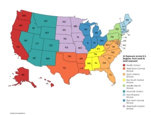
- Region – The U.S. region exposure rankings changed as well. For example, workers in the Pacific Division now experience the highest exposure, while those in the West North Central Division experience some of the lowest.
Interaction Effects
Lastly, I explored interactions — how two variables together might affect AI exposure differently than when considered separately — to explain the discrepancies between my initial and final results.
Example: Education & Income
When I looked at the effect of education and income on AI exposure independently, both showed positive relationships with AI exposure. However, once I included them together in the same model, a surprising shift occurred:
- Income remained positively associated with AI exposure
- Education’s effect became negative
This suggests that the earlier positive relationship between education and AI exposure was confounded by income. Education and income are strongly correlated, so in simpler models, education may have acted as a proxy for income. Once I controlled for income, however, the “true” effect of education became clear: among people with the same income, those with more education tend to have slightly lower AI exposure.
What’s Next?
Next week, I’ll wrap up my research by developing policy recommendations to address the inequalities I found in AI-related job displacement.
Thanks for following along! Please feel free to share any thoughts or questions in the comments—I’d love to hear them.
Comments:
All viewpoints are welcome but profane, threatening, disrespectful, or harassing comments will not be tolerated and are subject to moderation up to, and including, full deletion.