Week 10: How Many Clusters Are There?
Claire S -
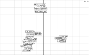
This week, I started actually analyzing the data. I used a lot of different tools this week that helped me figure out the relationships between the individuals. I started to use a software called RStudio, which is an environment where I can use the programming language R. The first analysis I did using RStudio used the program co-ancestry. This program looks at two individuals and estimates how related they are, with 0.0 being completely unrelated and 1 being identical twins- this means the samples came from the same individual. A value of 0.5 would correspond to a parent-child relationship or a sibling-sibling relationship- a value of 0.25 could also correspond to these relations. My data showed one pair with a value of 0.47, and after that, values were all less than 0.3.
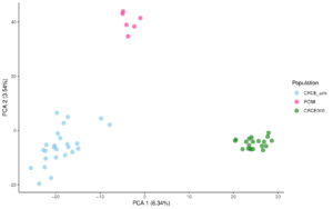
Next, I ran a principal component analysis (PCA), which reduces the dimensionality of the dataset. The program looks at the genetic variation within the dataset and estimates what percentage of it is caused by specific unknown variables called ‘principal components’ (PCs). I looked at the first two PCs since after that, the % caused by the PCs started to plateau. Then I created graphs that plotted the individuals against the principal components. This graph showed three clusters, which my mentors and I believe means there are three subpopulations. This is really exciting because it shows there could be some barriers to gene flow. The three clusters also make sense when thinking about our samples; each cluster came from a different area. (Graphs below)
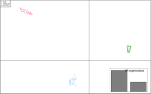
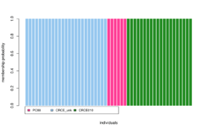
The next analysis I ran was called discriminant analysis of principal components (DAPC), which also identifies population structure. This analysis also showed the same three clusters, which was good. The DAPC also calculated the probability of each individual being in a certain cluster. (Graphs below).
I also ran populations, which I did last week, but this time the data included the three clusters. This allowed me to see the inbreeding values, the expected and observed heterozygosity of the clusters. I’ll use this data more to compare the genetic diversity of the clusters.
The last analysis I ran used the program LDNe, which estimates the effective population size. I’ll go over the results with my mentors on Monday.
This week, I learned that you get a lot of error messages when doing analyses, and that it takes a lot of problem-shooting. Next, I’ll start incorporating the geographic coordinates where the samples were collected. I’m excited to see what next week’s results show!
Comments:
All viewpoints are welcome but profane, threatening, disrespectful, or harassing comments will not be tolerated and are subject to moderation up to, and including, full deletion.