Week 7: Sensitivity Testing
Rohan V -
Hi all, it’s Rohan!
As I briefly mentioned last week, the new change point algorithm I’ve been working on over the last few weeks is just about finished. Now, I am able to apply it to experimental datasets that we generate in the lab! The results I’ve seen so far look promising; they will be covered in more detail in my final paper and presentation.
Today, I’ll be focusing on a unique method of scientific analysis which I was recently exposed to. This method is known as sensitivity testing, and it is a robust way to ensure that any results that one has obtained are due to physical differences in the data, rather than differences in how the data was handled. Sensitivity testing has been especially crucial for my project due to the highly stochastic (ie, highly variable) datasets that I am working with. But why is sensitivity testing essential for highly variable data?
To answer this question, I’ll delve into a bit of the math behind how points of structural change in datasets are detected in my change point detection (CPD) algorithm. Given a set of data (xn, yn), the CPD algorithm constructs a linear regression (ie, creates a line of best fit) to represent the entire dataset. It then calculates a sum of squared errors (SSE) for this linear regression, defined as the squared difference between the experimental values and the values predicted by the line of best fit.
After calculating the sum of squared errors for the individual line of best fit, the CPD algorithm proceeds to iterate through every single data point (x,y) in the set. It creates two lines of best fit split at the point that is being analyzed, and calculates the SSE for these linear regressions. CPD identifies a potential change point at the point (x,y) where the SSE is the smallest.
This process of splitting the data into more and more line segments can continue indefinitely, and the CPD algorithm can continue to find more changepoints. Here, however, it’s important to note that, assuming data is non-linear, splitting the data into more lines of best fit will always reduce the total SSE. Thus, to prevent ‘overfitting’ (where too many changepoints are identified for a given dataset), CPD adds a ‘penalty’ term for each additional change point that is detected. This process can be depicted in the equation below:
Total Cost J(k) = Sum of Squared Errors + βk
CPD considers a change point as valid when the addition of the change point, k, reduces the magnitude of the cost function, J(k). Here, the β term is known as the cost function coefficient: it is the penalty term which accompanies the detection of a change point.
Gaining an intuitive understanding of this equation helps in understanding the data which comes next. Let’s assume first that β is a relatively high value. In this case, if an additional change point is detected, the SSE goes down, but it is more than offset by the penalty term βk, resulting in the total cost J(k) increasing. Conversely, if β is a low value, then many more change points may be detected because the decrease in SSE is much greater in magnitude than the penalty term.
What is the implication of this equation? I manually control the β parameter, and the number of change points that are found depend on β. Thus, I conducted sensitivity tests to see how varying β affected the total number of change points detected in my data. In the graph below, the magnitude of the values is not important for understanding; the shape of the graph is.
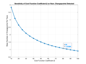
As shown in the image, at low β, the mean number of change points per set of (x,y) data analyzed is highly dependent on β. However, as β increases, we observe that the slope of the curve decreases significantly, conveying that for high β (>= 80), the mean number of change points detected is not highly dependent on the value of β. This confirmation is of immense value in the research community because it provides a way to ensure that one’s results are “real,” or, in other words, due to physically meaningful differences in data – rather than being due to user manipulation of inputs.
This result, which I have spent significant time coding over the past few weeks, guides me towards the optimal values for the cost function coefficient. As the project draws to a close, I’ll be placing the finishing touches on the results, analysis, and conclusion sections of my paper and creating my presentation; sensitivity testing will play a large role in both.
Thanks for tuning in!
Comments:
All viewpoints are welcome but profane, threatening, disrespectful, or harassing comments will not be tolerated and are subject to moderation up to, and including, full deletion.