Finding Clever Solutions, Week 9
Welcome back to my blog! This past week has seen a lot of progress on my Spike Sorting script. I am thankful I got the opportunity to meet with the original professor who made the same Matlab script. With my approach recalibrated, I found the first big inaccuracy of my code in the threshold filtration step.
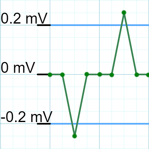
Explaining how it worked previously is quite simple. The script kept the data points with an absolute value greater than the threshold voltage set by the user, anything below the threshold stayed at a value of zero. I’ll refer to this old method as the binary “on-off” nature (Figure 1A and 1B).
Obviously the problem here is that the old process of keeping values above the threshold and setting the rest to zero does not preserve the entire waveform. I had observed the binary “on-off” nature in my previous version, and had chalked it up to the sampling rate deficiency in the hardware. I want to retract a statement I made in a previous blog about this hardware deficiency which was not at all causing the binary nature in the spiking data. Concluding that the sampling rate was responsible was a mistake, instead the underlying issue was in my filtration method.
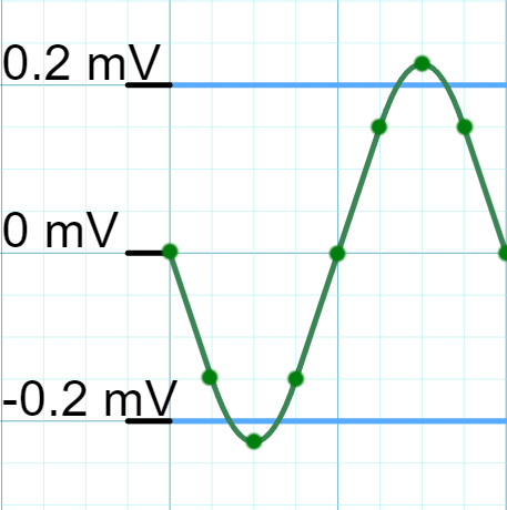
The newer filtration algorithm preserves the entire biphasic waveform. This could be a whole blog post in itself, but to summarize, the first step is identifying values above and below the threshold. In Figure 1B, this step would identify the five negative values below the threshold, and the five positive values above the threshold. I cluster these points together and extract that absolute maximum or minimum if it’s a positive or negative cluster. The next step I call “retrotracing” just means moving backwards from the negative peak to ensure all the points before are monotone increasing. The midtrace step also ensures the region between the negative and positive peak is monotone increasing. The last protrace is tracing past the positive peak to ensure that the last region is monotone decreasing. If all the regions are monotonically valid, the range of points identified is extracted as a valid spike for further analysis. This new method preserves the values that are below the threshold, but still part of the biphasic waveform.
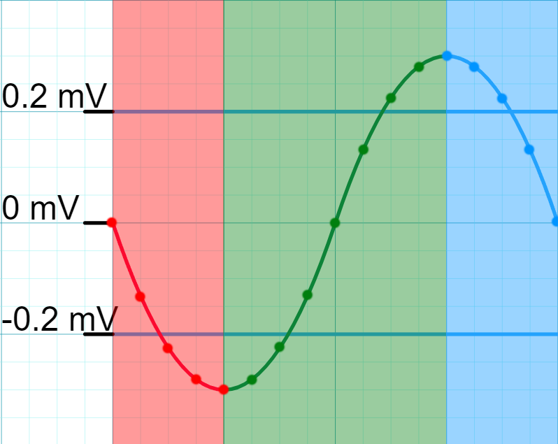
The last step of this new algorithm is linearly interpolating two waveform caps and a zero transition. Linear interpolation is a very complicated way to explain a basic algebra concept. To save myself an Algebra 1 tutorial, refer to the hastily drawn Figure 3. The essence is by manipulating the equation of a line, we can find the value of any point on that line. This is useful to generate the beginning and end caps or values at a clean zero value since the actual recording does not always start and end at zero but values slightly above or below that. I think linear interpolation is a very simple and clever solution.

The next steps to tackle are dimensionality reduction. Since each spike has varying lengths, I cannot simply apply Principal Component Analysis. One solution I am considering is interpolating the data to make all spikes uniform lengths without actually changing the data. Another possible solution I just came up with while writing this is to manually feature extract which would be now a lot easier with the full biphasic waveform, and apply PCA to that data frame.
This was a longer post but yet, a lot to compress. Each paragraph could be a whole blog post, so thank you for reading if you got this far. I look forward to sharing how I solve the aforementioned dimensionality reduction. See you next week!