Week 5: Utilizing Bayesian Updating for New Data
Ian M -
This week, I continued to focus on predicting future player performance using Bayesian methods. However, unlike last week, which focused on use of hierarchical data at a league-wide level, I focused on individual player data across several seasons. To make predictions using historical rather than hierarchical data, we have to use a different method known as Bayesian updating, one of the core aspects of Bayesian inference. The main components of my work this week involved learning what Bayesian updating was and how it could be used in the context of Francisco Lindor as he approached the middle of his career.
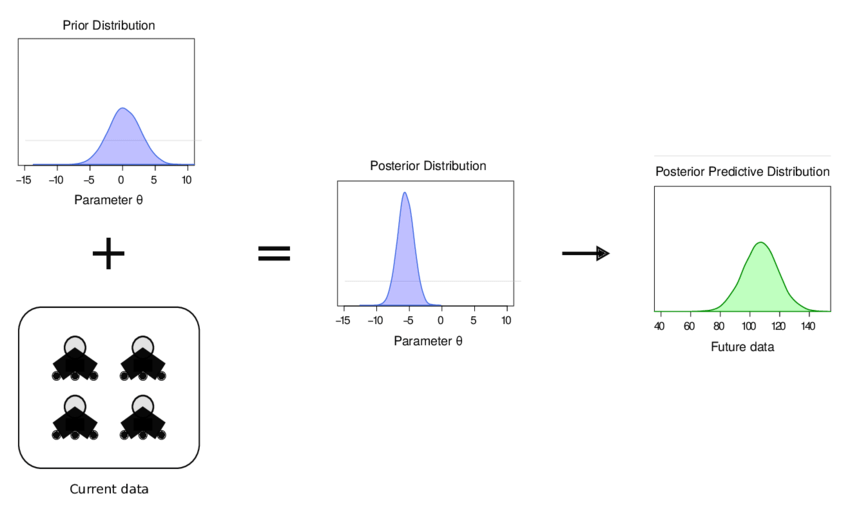
First off, Bayesian updating is a method for refining predictions by combining prior beliefs with new data using Bayes’ theorem to form posterior predictions for a given hypothesis or event. In the context of predicting a baseball player’s batting average, the prior is our initial estimate based on past performance, and the new data is the player’s current season statistics. Using Bayes’ Theorem, we update our belief about the player’s true batting average by calculating the likelihood of observing the current data given the prior. As more data is gathered, this process continuously improves the accuracy of our predictions, resulting in a more confident estimate of the player’s future performance as we shift our prior into a posterior predictive distribution.
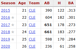
One useful example in the context of baseball can be found using Francisco Lindor as an example. Early on in Lindor’s career, his batting performance was consistently solid, with his .313 rookie batting average placing him at second for AL Rookie of the Year voting and consistently above .270 batting average earning him 4 consecutive All Star selections from 2016 to 2019. After the 2020 season, Lindor was set to become a free-agent in the upcoming season, so 2020 would be crucial to netting a large contract in the upcoming offseason. However, that year, his performance seemed to falter, with his batting average dropping to .258 in a shortened 2020 season. This raised concerns with Cleveland’s front office, who wondered if he was already regressing this early on in his career. Using Bayesian updating, we can determine if this season’s performance was statistically significant or not.
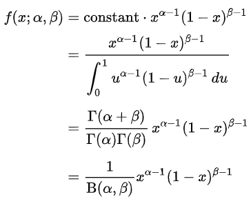
To set up a prior distribution for Bayesian updating, we need to create a beta distribution, a probability distribution based on a set of two positive parameters, to create a prior probability distribution for our data. A beta distribution can be defined by
and in our case,
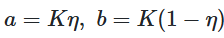
where η is our approximated prior mean and K is an approximation based on our level of confidence in our previous metrics. We can approximate η to approximately .280, since that was how Lindor performed prior to the 2020 season and through some experimentation, we find that K at 400 is a reasonable estimate given the number of at-bats he had to this point. Using these values, we find a is 112 and b is 288. With these, we can create a distribution that gives us both a prior beta distribution and a predictive posterior distribution that we can adjust based on the length of time we wish to use our data to predict.
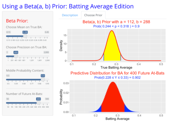
Based on our predictions here, we can see that the parameters of the posterior distribution did not shift to a significant degree compared to our prior distribution, suggesting that Lindor’s performance had not significantly changed during the 2020 season, implying that the results from that season may have just been randomness caused by a shortened season. Regardless, Cleveland would not reach an agreement on an extension for Lindor, who would instead sign a 10-year, $341 million contract extension with the Mets after a trade during the offseason. 2021 was a rough year for Lindor once again, as he would start off his season with a .218 batting average through the first three months of the season, having 58 hits in 265 at-bats. Using Bayesian updating once again, we can test if something notable has changed with his performance. This time, we begin with a and b rather than η and K, updating them by adding hits to a and non-hits to b.

This gives us a new posterior η of 0.256 and K of 665 by using the prior equations. With this new update to our distributions, we can now chart our new prior distribution and our new posterior distribution.
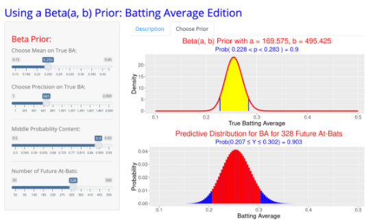
From this data, we can notice that our parameters have shifted noticeably downwards compared to our previous distributions, with our confidence and credible intervals having shifted downwards to a noticeable degree. Due to this shift, we can determine that some external factor has negatively impacted his performance. In the case of older players, such regression is often just aging, but Lindor was still quite young, so that was unlikely. Instead, what had happened was an oblique strain that he suffered early on in the season that he had been playing through. Due to this, he would miss about a month and a half of the season healing from his injury, and after doing so, his performance bounced back massively, returning to his pre-2019 form and even finishing second in NL MVP voting in 2024. By using Bayesian statistics, we were able to notice that while Lindor’s batting average decline in 2020 may have just been purely random, his decline in early 2021 was not random and was instead caused by an injury. Through Bayesian updating, we can update our datasets and parameters in real time as a baseball player plays in a season to identify more subtle patterns and changes in data over time.
Comments:
All viewpoints are welcome but profane, threatening, disrespectful, or harassing comments will not be tolerated and are subject to moderation up to, and including, full deletion.