It’s in Fortran???
Daniel j -
As much as I love reading about the theoretical aspects of my project, I must also consider how to apply that theory to give it a physical form. So, as all engineers must do at some point, I turned to computer science.
Starting off, even with my background in coding, especially with Python and Java, I struggled to understand the sample simulation code I was given to familiarize myself with the project. Following the code was a little overwhelming, especially given that much of the script was in Fortran and MATLAB script. On top of that, many of the files had confusing names as well as unnecessary bits of code.
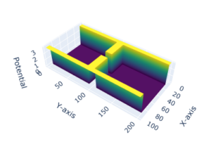
Working with Mr. Gil Speyer, a research accelerator at ASU, I gained access to the Sol supercomputer and learned how to navigate the simulation platform that utilized it. There, I slowly worked through the introductory code, testing the simulations myself through MATLAB. After a few hours of reading through research papers and studying the code and its outputs, I came to learn that what it created was a potential graph and transmission graph of a modded quantum wire (shown below).
What you see in the first graph is the geometry of a quantum wire with a well going across it. It creates these by using something called a “mesh,” where an area is divided into grid points (this is possible because of the 2D electron layer that the MoS2 semiconductor creates), which are each assigned certain potential values. The second shows how transmission behaves according to different gate voltage/Fermi energy values, where the step-like nature of this graph is a reflection of conductance quantization, or the idea that the transmission changes only when certain energy levels are reached.
After my introduction to simulation coding and the theory behind it, Professor Vasileksa proposed that given my familiarity with Python, I develop the code in Jupyter, where I could use Python and the visualization tools it offered. So, I got started right away.
The first task I was given was to create the geometry for a simple quantum point contact. Using the guidance of the Fortran code, I used familiar Python modules as well as newly learned ones to create the following visualization in Jupyter:
Now, using this start, I must now create other geometries (not just the quantum point contact, but also others like quantum dots), find a way to link and visualize the transmission graph using the Usuki calculation method, and add user-interactive features to make it more flexible (i.e., adjustable mesh size, quantum point contact gap size, etc.).
In my recent meetings with Professor Vasileska and her team, we have talked about our end goal of creating a Graphical User Interface (GUI) on nanoHUB, where users can choose different geometries and input settings to see the transmission graph output as well as an electron density graph output (this will be discussed in a later blog).
As I move on to the following week, I am excited to implement new features into my code and learn more about the simulation process.
Comments:
All viewpoints are welcome but profane, threatening, disrespectful, or harassing comments will not be tolerated and are subject to moderation up to, and including, full deletion.